In this project, I evaluated the performance and predictive power of a model that has been trained and tested on data collected from homes in suburbs of Boston, Massachusetts. A model trained on this data that is seen as a good fit could then be used to make certain predictions about a home — in particular, its monetary value. This model would prove to be invaluable for someone like a real estate agent who could make use of such information on a daily basis.
The dataset for this project originates from the UCI Machine Learning Repository. The Boston housing data was collected in 1978 and each of the 506 entries represent aggregated data about 14 features for homes from various suburbs in Boston, Massachusetts. For the purposes of this project, the following preprocessing steps have been made to the dataset:
- 16 data points have an
'MEDV'value of 50.0. These data points likely contain missing or censored values and have been removed. - 1 data point has an
'RM'value of 8.78. This data point can be considered an outlier and has been removed. - The features
'RM','LSTAT','PTRATIO', and'MEDV'are essential. The remaining non-relevant features have been excluded. - The feature
'MEDV'has been multiplicatively scaled to account for 35 years of market inflation.
The code cell below loads the Boston housing dataset, along with a few of the necessary Python libraries required for this project. The dataset loaded successfully and the size of the dataset is reported.
# Import libraries necessary for this project
import numpy as np
import pandas as pd
import visuals as vs # Supplementary code
from sklearn.cross_validation import ShuffleSplit

# Pretty display for notebooks
%matplotlib inline

# Load the Boston housing dataset
data = pd.read_csv('housing.csv')
prices = data['MEDV']
features = data.drop('MEDV', axis = 1)

# Success
print "Boston housing dataset has {} data points with {} variables each.".format(*data.shape)
Boston housing dataset has 489 data points with 4 variables each.
Data Exploration
In this first section of this project, I will make a cursory investigation about the Boston housing data and provide the observations. Familiarizing myself with the data through an explorative process is a fundamental practice to help me better understand and justify my results.
Since the main goal of this project is to construct a working model which has the capability of predicting the value of houses, we will need to separate the dataset into features and the target variable. The features, 'RM', 'LSTAT', and 'PTRATIO', give us quantitative information about each data point. The target variable, 'MEDV', will be the variable we seek to predict. These are stored in features and prices, respectively.
Implementation: Calculate Statistics
For my very first coding implementation, I will calculate descriptive statistics about the Boston housing prices. Since numpy has already been imported, use this library to perform the necessary calculations. These statistics will be extremely important later on to analyze various prediction results from the constructed model.
In the code cell below, I will need to implement the following:
- Calculate the minimum, maximum, mean, median, and standard deviation of
'MEDV', which is stored inprices.- Store each calculation in their respective variable.
# TODO: Minimum price of the data
minimum_price = np.min(prices)

# TODO: Maximum price of the data
maximum_price = np.max(prices)

# TODO: Mean price of the data
mean_price = np.mean(prices)

# TODO: Median price of the data
median_price = np.median(prices)

# TODO: Standard deviation of prices of the data
std_price = np.std(prices)

# Show the calculated statistics
print "Statistics for Boston housing dataset:\n"
print "Minimum price: ${:,.2f}".format(minimum_price)
print "Maximum price: ${:,.2f}".format(maximum_price)
print "Mean price: ${:,.2f}".format(mean_price)
print "Median price ${:,.2f}".format(median_price)
print "Standard deviation of prices: ${:,.2f}".format(std_price)
Statistics for Boston housing dataset:

Minimum price: $105,000.00
Maximum price: $1,024,800.00
Mean price: $454,342.94
Median price $438,900.00
Standard deviation of prices: $165,171.13
Question 1 - Feature Observation
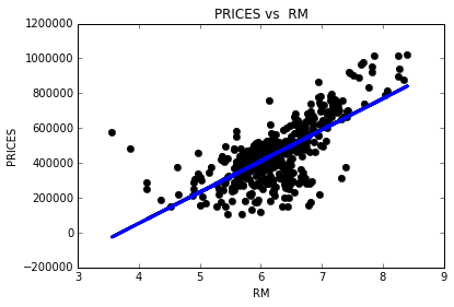
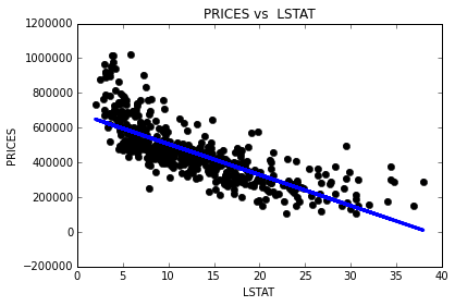
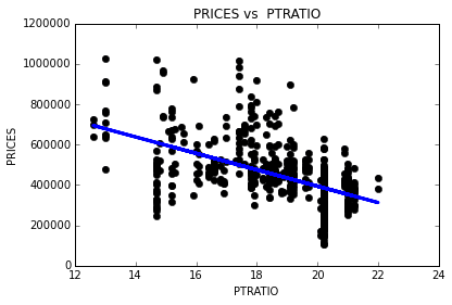
As a reminder, we are using three features from the Boston housing dataset: 'RM', 'LSTAT', and 'PTRATIO'. For each data point (neighborhood):
'RM'is the average number of rooms among homes in the neighborhood.'LSTAT'is the percentage of homeowners in the neighborhood considered “lower class” (working poor).'PTRATIO'is the ratio of students to teachers in primary and secondary schools in the neighborhood.
import matplotlib.pyplot as plt
import numpy as np

for col in features.columns:

    fig, ax = plt.subplots()
    fit = np.polyfit(features [col], prices, deg=1) # We use a linear fit to compute the trendline
    ax.scatter(features [col],  prices)
    plt.plot(features [col], prices, 'o', color='black')
    ax.plot(features[col], fit[0] * features[col] + fit[1], color='blue', linewidth=3) # This plots a trendline with the regression parameters computed earlier. We should plot this after the dots or it will be covered by the dots themselves
    plt.title('PRICES vs  '+ str(col)) # title here
    plt.xlabel(col) # label here
    plt.ylabel('PRICES') # label here
**Answer: **
1) I expect that higher ‘RM’ value would lead to an increase in the value of ‘MEDV’. Usually, larger houses have more rooms and have higher prices.
2) I expect that there is negative correlation between the ‘LSTAT’ and the ‘MEDV’. If the percentage of “lower class” in the neighborhood is high, there are low-priced housing. Because most people live in affordable places because they need to pay for taxes, rent, and so on.
3) I think the ‘PTRATIO’ and the ‘MEDV’ have positive correlation. The reason is that people living in expensive area can affect the ratio of students to teachers in that area. Property taxtation and school funding are closely linked in United States, so schools with better financial condition can increase the ratio of students to teachers. Paying more perperty taxes means having more assets, therefore I expect the house prices of those people are high.
Developing a Model
In this second section of the project, I developed the tools and techniques necessary for a model to make a prediction. Being able to make accurate evaluations of each model’s performance through the use of these tools and techniques helps to greatly reinforce the confidence in my predictions.
Implementation: Define a Performance Metric
It is difficult to measure the quality of a given model without quantifying its performance over training and testing. This is typically done using some type of performance metric, whether it is through calculating some type of error, the goodness of fit, or some other useful measurement. For this project, I calculated the coefficient of determination, R2, to quantify my model’s performance. The coefficient of determination for a model is a useful statistic in regression analysis, as it often describes how “good” that model is at making predictions.
The values for R2 range from 0 to 1, which captures the percentage of squared correlation between the predicted and actual values of the target variable. A model with an R2 of 0 always fails to predict the target variable, whereas a model with an R2 of 1 perfectly predicts the target variable. Any value between 0 and 1 indicates what percentage of the target variable, using this model, can be explained by the features. A model can be given a negative R2 as well, which indicates that the model is no better than one that naively predicts the mean of the target variable.
For the performance_metric function in the code cell below, I implemented the following:
- Used
r2_scorefromsklearn.metricsto perform a performance calculation betweeny_trueandy_predict. - Assigned the performance score to the
scorevariable.
# Import 'r2_score'
from sklearn.metrics import r2_score
def performance_metric(y_true, y_predict):
    """ Calculates and returns the performance score between
        true and predicted values based on the metric chosen. """

    # Calculate the performance score between 'y_true' and 'y_predict'
    score = r2_score(y_true, y_predict)

    # Return the score
    return score
Question 2 - Goodness of Fit
Assume that a dataset contains five data points and a model made the following predictions for the target variable:
Table 1: Example data points and predictions
| True Value | Prediction |
|---|---|
| 3.0 | 2.5 |
| -0.5 | 0.0 |
| 2.0 | 2.1 |
| 7.0 | 7.8 |
| 4.2 | 5.3 |
Would I consider this model to have successfully captured the variation of the target variable? Why or why not?
The code cell below used the performance_metric function to calculate the model’s coefficient of determination.
# Calculate the performance of this model
score = performance_metric([3, -0.5, 2, 7, 4.2], [2.5, 0.0, 2.1, 7.8, 5.3])
print "Model has a coefficient of determination, R^2, of {:.3f}.".format(score)
Model has a coefficient of determination, R^2, of 0.923.
Answer: R2 shows performance of my model by capturing percentage of squared correlation between the predicted and actual values of the target variable. It is close to 1, so I can say that this model predicts quite accurately.
Implementation: Shuffle and Split Data
I took the Boston housing dataset and splitted the data into training and testing subsets. Typically, the data is also shuffled into a random order when creating the training and testing subsets to remove any bias in the ordering of the dataset.
For the code cell below, I implemented the following:
- Used
train_test_splitfromsklearn.cross_validationto shuffle and splitted thefeaturesandpricesdata into training and testing sets.- Splitted the data into 80% training and 20% testing.
- Set the
random_statefortrain_test_splitto a value of my choice. This ensures results are consistent.
- Assigned the train and testing splits to
X_train,X_test,y_train, andy_test.
# Import 'train_test_split'
from sklearn.cross_validation import train_test_split

# Shuffle and split the data into training and testing subsets
X_train, X_test, y_train, y_test = train_test_split(features, prices, test_size=0.2, random_state=0)

# Success
print "Training and testing split was successful."
Training and testing split was successful.
Question 3 - Training and Testing
What is the benefit to splitting a dataset into some ratio of training and testing subsets for a learning algorithm?
**Answer: ** Spliting training and testing data gives estimate of performance on an independent dataset. Also, it serves as check on overfitting, which is high variance in the model. Without test data, we can’t sure our model can predict accurately when our model is fed unseen data.
Analyzing Model Performance
In this third section of the project, I looked at several models’ learning and testing performances on various subsets of training data. Additionally, I investigated one particular algorithm with an increasing 'max_depth' parameter on the full training set to observe how model complexity affects performance. Graphing my model’s performance based on varying criteria can be beneficial in the analysis process, such as visualizing behavior that may not have been apparent from the results alone.
Learning Curves
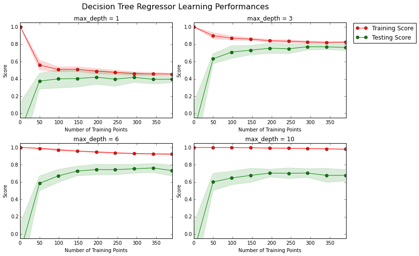
The following code cell produces four graphs for a decision tree model with different maximum depths. Each graph visualizes the learning curves of the model for both training and testing as the size of the training set is increased. Note that the shaded region of a learning curve denotes the uncertainty of that curve (measured as the standard deviation). The model is scored on both the training and testing sets using R2, the coefficient of determination.
# Produce learning curves for varying training set sizes and maximum depths
vs.ModelLearning(features, prices)
Question 4 - Learning the Data
Choose one of the graphs above and state the maximum depth for the model. What happens to the score of the training curve as more training points are added? What about the testing curve? Would having more training points benefit the model?
**Answer: ** Let’s look at a graph with max_depth=3. As training points are added, training curve converges to about 0.8 after 150 training points. And testing scores also converges at similar value 0.8. Thus, having more training points would not benifit the model.
Complexity Curves
The following code cell produces a graph for a decision tree model that has been trained and validated on the training data using different maximum depths. The graph produces two complexity curves — one for training and one for validation. Similar to the learning curves, the shaded regions of both the complexity curves denote the uncertainty in those curves, and the model is scored on both the training and validation sets using the performance_metric function.
vs.ModelComplexity(X_train, y_train)
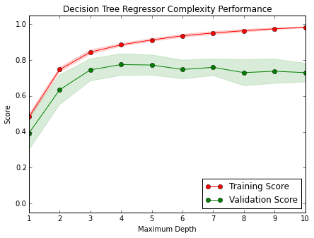
Question 5 - Bias-Variance Tradeoff
When the model is trained with a maximum depth of 1, does the model suffer from high bias or from high variance? How about when the model is trained with a maximum depth of 10? What visual cues in the graph justify my conclusions?
**Answer: ** In case of maximum depth of 1, the model suffer from high bias. Because both of them have a low score, and it means the model does not represent the underlying relationship.
In case of maximum depth of 10, there are huge gaps between two curves, and I barely see testing curve. In this case, the model suffer from an over-fitting probelm(high variance).
Question 6 - Best-Guess Optimal Model
Which maximum depth do I think results in a model that best generalizes to unseen data? What intuition lead me to this answer?
**Answer: ** I think maximum depth of 3 results in the best model. Both the training and testing curves converge at around 0.8. There is smaller gap between the training and testing sets than other graphs, which means this model generalizes well. In addition, higher converging core means that better our model performs.
Evaluating Model Performance
In this final section of the project, I constructed a model and made a prediction on the client’s feature set using an optimized model from fit_model.
Question 7 - Grid Search
What is the grid search technique and how it can be applied to optimize a learning algorithm?
**Answer: ** GridSearchCV is a way of systematically working through multiple combinations of parameter tunes. It exhaustively search over specified parameter values for a learning algorithm. Thus we can determine which tune gives the best performance.
There are other techniques that could be used for hyperparameter optimization in order to save time like RandomizedSearchCV, in this case instead of exploring the whole parameter space just a fixed number of parameter settings is sampled from the specified distributions. This proves useful when we need to save time but is not necessary in cases in cases like ours where the data set is relatively small.
Question 8 - Cross-Validation
What is the k-fold cross-validation training technique? What benefit does this technique provide for grid search when optimizing a model?
**Answer: ** K-fold CV training technique splits data points into k bins, and pick one of those bins as a testing data, and others as training data, then iterate validation k times. Then the average error across all k trials is computed. The advantage of this method is that it matters less what combination of parameters is used and how the data gets divided. Every data point and parameter combination gets to be in a test set exactly once, and gets to be in a training set k-1 times. The variance of the resulting estimate is reduced as k is increased. Therefore, it ensures assessment of model whether tuned parameters actually gives best performance.
I refered Cross Validation.
Implementation: Fitting a Model
The final implementation trained a model using the decision tree algorithm. To ensure that I produced an optimized model, I trained the model using the grid search technique to optimize the 'max_depth' parameter for the decision tree. The 'max_depth' parameter can be thought of as how many questions the decision tree algorithm is allowed to ask about the data before making a prediction. Decision trees are part of a class of algorithms called supervised learning algorithms.
For the fit_model function in the code cell below, I implemented the following:
- Used
DecisionTreeRegressorfromsklearn.treeto create a decision tree regressor object.- Assigned this object to the
'regressor'variable.
- Assigned this object to the
- Created a dictionary for
'max_depth'with the values from 1 to 10, and assign this to the'params'variable. - Useed
make_scorerfromsklearn.metricsto create a scoring function object.- Passed the
performance_metricfunction as a parameter to the object. - Assigned this scoring function to the
'scoring_fnc'variable.
- Passed the
- Used
GridSearchCVfromsklearn.grid_searchto create a grid search object.- Passed the variables
'regressor','params','scoring_fnc', and'cv_sets'as parameters to the object. - Assigned the
GridSearchCVobject to the'grid'variable.
- Passed the variables
# TODO: Import 'make_scorer', 'DecisionTreeRegressor', and 'GridSearchCV'
from sklearn.tree import DecisionTreeRegressor
from sklearn.metrics import make_scorer
from sklearn.grid_search import GridSearchCV
from sklearn.cross_validation import ShuffleSplit

def fit_model(X, y):
    """ Performs grid search over the 'max_depth' parameter for a
        decision tree regressor trained on the input data [X, y]. """

    # Create cross-validation sets from the training data
    cv_sets = ShuffleSplit(X.shape[0], n_iter = 10, test_size = 0.20, random_state = 0)

    # TODO: Create a decision tree regressor object
    regressor = DecisionTreeRegressor()

    # TODO: Create a dictionary for the parameter 'max_depth' with a range from 1 to 10
    params = {'max_depth': np.arange(1,11)}

    # TODO: Transform 'performance_metric' into a scoring function using 'make_scorer'
    scoring_fnc = make_scorer(performance_metric)

    # TODO: Create the grid search object
    grid = GridSearchCV(regressor, cv=cv_sets, param_grid= params, scoring=scoring_fnc)

    # Fit the grid search object to the data to compute the optimal model
    grid = grid.fit(X, y)

    # Return the optimal model after fitting the data
    return grid.best_estimator_
Making Predictions
Once a model has been trained on a given set of data, it can now be used to make predictions on new sets of input data. In the case of a decision tree regressor, the model has learned what the best questions to ask about the input data are, and can respond with a prediction for the target variable. I can use these predictions to gain information about data where the value of the target variable is unknown — such as data the model was not trained on.
Question 9 - Optimal Model
What maximum depth does the optimal model have? How does this result compare to my guess in Question 6?
The code block below fits the decision tree regressor to the training data and produces an optimal model.
# Fit the training data to the model using grid search
reg = fit_model(X_train, y_train)

# Produce the value for 'max_depth'
print "Parameter 'max_depth' is {} for the optimal model.".format(reg.get_params()['max_depth'])
Parameter 'max_depth' is 4 for the optimal model.
**Answer: ** ‘max_depth’ is 4 for the optimal model. The result is close to my guess that ‘max_depth’ of 3 would be the best.
Question 10 - Predicting Selling Prices
If a real estate agent in the Boston area looking to use this model to help price homes owned by clients that they wish to sell. Suppose I collected the following information from three of clients:
Table 2: House information from three of clients
| Feature | Client 1 | Client 2 | Client 3 |
|---|---|---|---|
| Total number of rooms in home | 5 rooms | 4 rooms | 8 rooms |
| Neighborhood poverty level (as %) | 17% | 32% | 3% |
| Student-teacher ratio of nearby schools | 15-to-1 | 22-to-1 | 12-to-1 |
What price would I recommend each client sell his/her home at? Do these prices seem reasonable given the values for the respective features?
The code block below has the optimized model makes predictions for each client’s home.
# Produce a matrix for client data
client_data = [[5, 17, 15], # Client 1
               [4, 32, 22], # Client 2
               [8, 3, 12]]  # Client 3

# Show predictions
for i, price in enumerate(reg.predict(client_data)):
    print "Predicted selling price for Client {}'s home: ${:,.2f}".format(i+1, price)
Predicted selling price for Client 1's home: $391,183.33
Predicted selling price for Client 2's home: $189,123.53
Predicted selling price for Client 3's home: $942,666.67
**Answer: ** I predicted selling prices and described these prices along with the earlier calculated descriptive statistics.
- Predicted selling price for Client 1’s home: $391,183.33
- This house is slightly cheaper than average house price, and it falls inside the range of standard deviation of house prices.
- Predicted selling price for Client 2’s home: $189,123.53
- This price is in low-percentile of house prices.
- Predicted selling price for Client 3’s home: $942,666.67
- This price falls in high-percentile of house prices, because it is close to maximum price.
I expected more rooms, lower student-teacher ratio, lower neighborhood poverty level lead to higher prices. The prediction is correspond with my expectation.
Sensitivity
An optimal model is not necessarily a robust model. Sometimes, a model is either too complex or too simple to sufficiently generalize to new data. Sometimes, a model could use a learning algorithm that is not appropriate for the structure of the data given. Other times, the data itself could be too noisy or contain too few samples to allow a model to adequately capture the target variable — i.e., the model is underfitted. Run the code cell below to run the fit_model function ten times with different training and testing sets to see how the prediction for a specific client changes with the data it’s trained on.
vs.PredictTrials(features, prices, fit_model, client_data)
Trial 1: $391,183.33
Trial 2: $419,700.00
Trial 3: $415,800.00
Trial 4: $420,622.22
Trial 5: $413,334.78
Trial 6: $411,931.58
Trial 7: $399,663.16
Trial 8: $407,232.00
Trial 9: $351,577.61
Trial 10: $413,700.00

Range in prices: $69,044.61
Question 11 - Applicability
In a few sentences, discuss whether the constructed model should or should not be used in a real-world setting.
There are some questions to answering:
- How relevant today is data that was collected from 1978?
- Are the features present in the data sufficient to describe a home?
- Is the model robust enough to make consistent predictions?
- Would data collected in an urban city like Boston be applicable in a rural city?
**Answer: ** The feature ‘MEDV’ has been multiplicatively scaled to account for 35 years of market inflation, so this model might be used to predict today’s house prices. However, the original data has more features which can represent various aspect of house prices. For example, ‘DIS’ (weighted distances to five Boston employment centres) might influence prices since people are willing to pay higher price for commuting in shorter distance. ‘CRIM’ (per capita crime rate by town) might be important because people pay more to have secure neighborhood. In addition, we need to consider other factors that may not be available 35 years ago or changed during that time. For instance, new roads could be constructed which can affect commuting convenience.
After training and testing 10 times, I got fairly robust prediction because prices range was $69,044.61 which is smaller amount of money than cheapest house ($105,000.00). It is included in one standard deviation range($165,171.13) from the mean. But, we need to be careful when we apply this model in a rural city. Houses in the rural area have different aspect, so investigation of new features and corresponding data points are needed to make price model for the rural city.
I also tried to find the nearest neighbours of the feature vector. Then I could contrast the results with the closest neighbours, the ones that have similar characteristics.
from sklearn.neighbors import NearestNeighbors
num_neighbors=5
def nearest_neighbor_price(x):
    def find_nearest_neighbor_indexes(x, X):  # x is my vector and X is the data set.
        neigh = NearestNeighbors( num_neighbors )
        neigh.fit(X)
        distance, indexes = neigh.kneighbors( x )
        return indexes
    indexes = find_nearest_neighbor_indexes(x, features)
    sum_prices = []
    for i in indexes:
        sum_prices.append(prices[i])
    neighbor_avg = np.mean(sum_prices)
    return neighbor_avg
index = 0
for i in client_data:
    val=nearest_neighbor_price(i)
    index += 1
    print "The predicted {} nearest neighbors price for home {} is: ${:,.2f}".format(num_neighbors,index, val)
The predicted 5 nearest neighbors price for home 1 is: $372,540.00
The predicted 5 nearest neighbors price for home 2 is: $162,120.00
The predicted 5 nearest neighbors price for home 3 is: $897,120.00